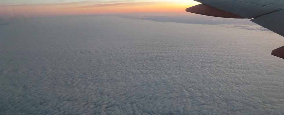
Clouds have complex structures even at very small spatial scale, varying second by second (Fig. 1). The small-scale variability of cloud influences radiative transfer and radiation observed from satellites. However, numerical models cannot treat the variability at infinitesimal scale, so idealized cloud morphology should be used.
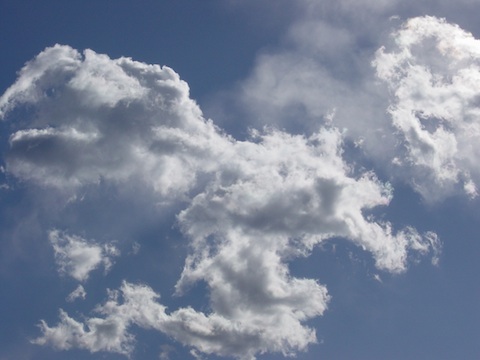
Fig. 1. A photo of fair weather cumulus.
Our group is developing 3D radiative transfer models with purposes of understanding of the 3D radiative effects in an atmosphere with inhomogeneous clouds, interpretation of various observation data, and development of improved remote sensing techniques. One of such models is MCARaTS (Monte Carlo Atmospheric Radiative Transfer Simulator), which is a general-purpose model to treat the unpolarized radiative transfer in the system of atmosphere, ocean and land at narrow bands in a spectrum from UV to microwave. In the model, we take into account the light scattering by cloud, aerosol, and air molecules and reflection by water and land surfaces. The Monte Carlo photon-tracing method is used. Many model photons are emitted from the radiative sources, and the position and direction of scattering are determined by random numbers (Fig. 2). The radiative flux and heating rate are estimated by accumulating the photon energy. The computer code is parallelized so as to run efficiently on a large-scale computer (e..g, supercomputer). The model is summarized in Table 1.
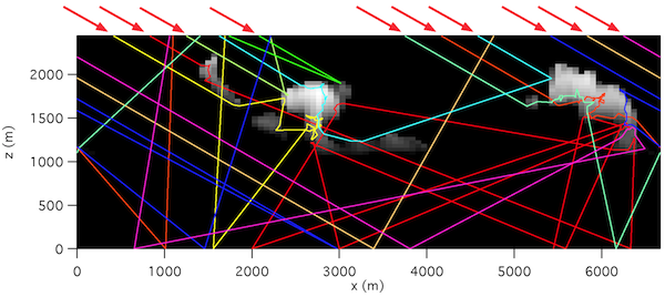
Fig. 2. An example of photon trajectories simulated by the Monte Carlo photon tracing algorithm.
Table 1. Summary of the 3D radiative transfer model MCARaTS.
| Coordinate system | 3D Cartesian |
| Radiative sources | Solar radiation and thermal emission |
| Physical processes | Scattering and absorption by air molecules, aerosols, and hydrometeors |
| Surface reflection | Semi-empirical BRDFs of water and land surfaces |
| Radiative transfer solution algorithm | The forward-propagating Monte Carlo photon-tracing algorithm |
| Radiative quantities calculated | Radiative flux (direct/diffuse), radiative heating rate, radiance, and pathlength distribution |
An example of computed solar reflectance of cloud is shown in Fig. 3. We assumed a stratocumulus cloud deck with an average thickness of 300 m. The figure represents high horizontal resolution images of nadir reflectance at visible and near-infrared wavelengths. The single scattering albedo (ω0) denotes the fraction of scattering to extinction. When ω0 = 1, the particles exhibit no absorption, and this is the situation in the visible. Weak absorption (ω0 = 0.96-0.99) is representative in the near-infrared. Large differences are shown between 3D and 1D radiative transfers, where 1D computations are obtained by solving 1D radiative transfer equations independently for atmospheric columns. When the solar zenith angle (θ0) is 0˚, the “3D” image is smoother than those of 1D. The smoothing effect is strong when the absorption is weak (ω0 = 1). When θ0 = 60˚, the smoothing is still apparent. However, an opposite effect, roughening, appears at spatial scale of about 1 km, so that the reflectance variability is enhanced.
Although MCARaTS is for calculations at monochromatic wavelengths or narrowbands, a simplified broadband radiative transfer model (code name: SORASCAT) is now under development for efficient 3D radiative transfer simulations for a large number of time-steps.
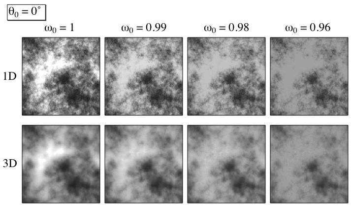

Fig. 3. Simulated satellite observation images with high horizontal resolution. A stratocumulus cloud deck with an average thickness of 300 m was assumed. These images represent solar reflectances at wavelengths in the visible and near-infrared spectra. The horizontal resolution is 50 m, and the one side of the entire square region is 6.4 km. The single scattering albedo is denoted by ω0, and the solar zenith angles by θ0.